Guidance On Carrying Out A TM54 Assessment in Tas
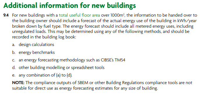
TM54’s are being carried out on buildings more frequently and it’s likely this will continue to be the case with the new edition of ‘Part L: Conservation of Fuel & Power’ document coming into effect on 15th June 2022. The reason for this is the new requirement for buildings with a useful floor area of over 1000m2 requiring a forecast of actual energy use at handover, as outlined in section 9.4:
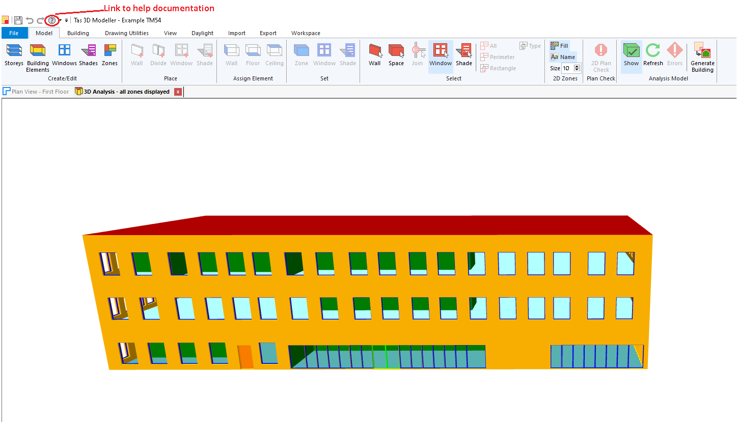
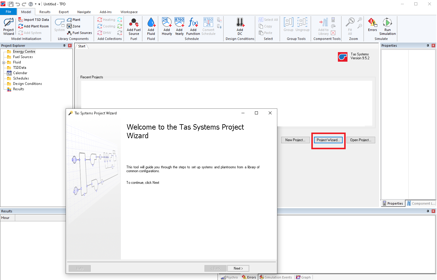
We’ve put together a worked example of a fairly simple TM54 to show you the process of carrying one out in Tas – as TM54 is an in depth analysis it is assumed you already have good knowledge on using Tas and won’t go into great detail on things like using the 3D modeller. If you feel you’re struggling to follow the worked example or want more detail on some of the steps carried out we recommend that you look at the help documentation for these specific areas. Help can be accessed through the Tas Manager or from the help icon in each application (as highlighted in the below screenshot of the example building) or by pressing the F1 key.
We are offering in person training in our office again and if you’re interested in booking onto one of our courses on how to use Tas you can do so on our website here. If you would like to know more about the TM54 assessment in general or the benefits of carrying one out on your building, check out our previous blog on TM54.
It is of course highly recommended that TM54 is read in conjunction with this worked example as we won’t go into great detail on the guidance already given in this or on how exactly the results should be reported. The aim of this example is to show you how to set up a Tas model correctly to provide you with the predicted energy usage of a building. The worked example will look at creating a central case or baseline model first and then outline how scenario modelling for error margins could be done. If you would like to purchase a copy of TM54 you can do so from CIBSEs website here
Setting up the T3D and introducing the building.
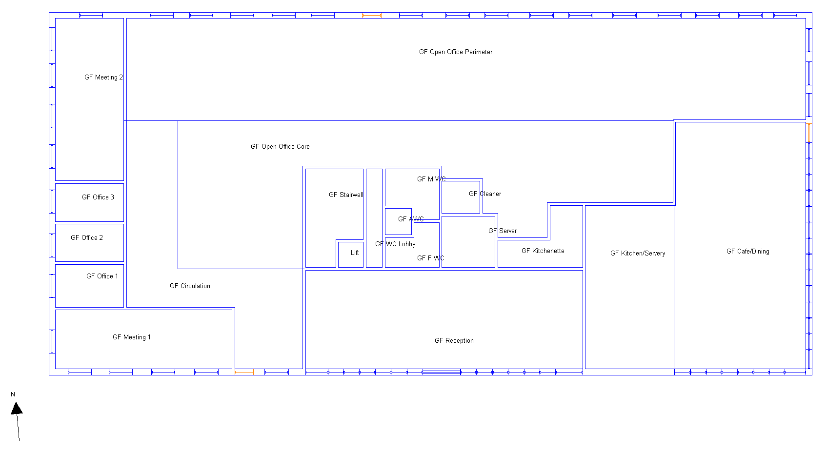
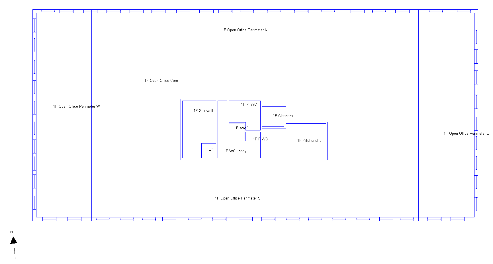
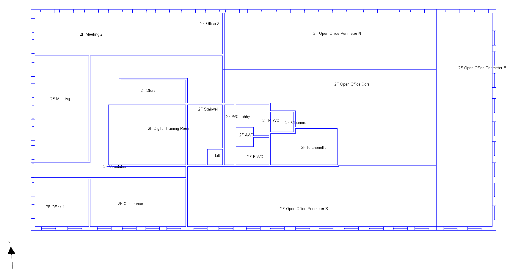
The building we are using for this example is a fairly standard office building with a kitchen and café on the ground floor. When zoning your building you should ensure that all spaces to be included in the TM54 analysis have been zoned. In some cases the zones will need to be split up into smaller zones, this is the case for our open office spaces as only the perimeter of the open offices have daylight dimming controls on the lighting.It is expected that the TM54 wont be the first analysis done on the building in Tas, it is likely an overheating, loads calculation or compliance model has already been done, so we can use any of those assessments as our starting point and edit them as necessary for our TM54. Here are the floor plans for the building:
GF
1F
2F
As with all Tas models if you have more than one construction type for a building element (e.g. a lightweight external wall and a brick external wall) then these should be split up in the T3D so that the correct construction can be assigned in the TBD. It’s also important that the correct Floor-ceiling heights are modelled, this can be done by ensuring ceiling and floor elements with the correct building element thickness are used.
Setting up the TBD
The calendar assigned in the TBD should account for when the building is closed, this includes public holidays such as the Easter and Christmas period. Our building is closed over weekends and public holidays but open on all other weekdays so the ‘NCM Standard’ calendar is being used.
TM54 states that an appropriate weather set should be used for the assessment, as such we’re going to be using the CIBSE Birmingham 2020 high emissions 50th percentile TRY weather file.
HVAC groups should be created for each HVAC system and all zones to be included in the analysis should be assigned to the appropriate HVAC group, these will be used in Tas systems when setting up/amending the Systems. Whilst this isn’t mandatory it will make things a lot easier when it comes to setting up and editing systems.
Setting up the internal conditions for the TM54 is what requires most work in the TBD, the internal conditions assigned should reflect the actual building, and this should include any out of hour’s usage that should be accounted for. Let’s go through setting up each bit separately:
Infiltration – This one’s fairly straightforward, just set up the infiltration in air changes per hour for each space. This can be inferred from CIBSE Guide A Infiltration tables, based on the expected Air Permeability of the building.
Ventilation – Mechanical ventilation should be included here, any mechanical ventilation included in the internal condition will be provided to the space at outside air conditions. The mechanical ventilation can be set up in more detail later on when we create the Tas Systems file, where it can be tempered and heat recovery can be included.
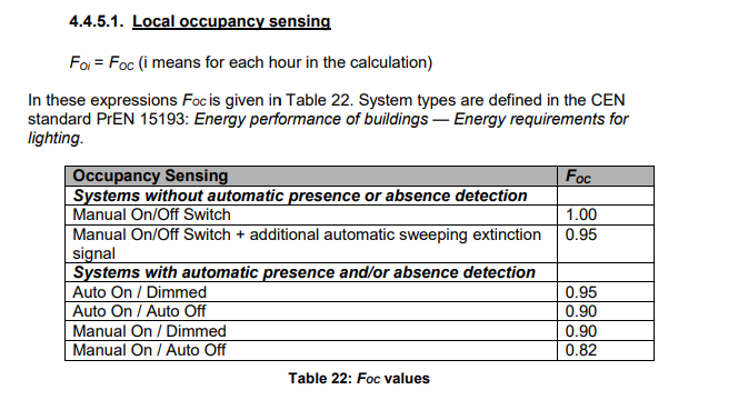
Lighting Gain – The lighting gain modelled should reflect the actual W/m2 values for each space if this information is available, lighting gains can be set on a schedule so that they’re off for hours where the room isn’t expected to be occupied. If spaces have presence or absence detection control, the reduction in lighting usage can be accounted for by applying a factor to the W/m2 value used, if you’re unsure what factor to use a good starting point could be looking at table 22 in the SBEM technical manual:
Daylight linked lighting control should be accounted for by applying a function to the lighting gain, our perimeter office spaces have photocell dimming control so let’s set this up for a space:
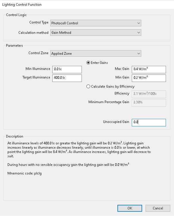
The minimum illuminance is the lowest lighting level the lights can provide to the space, the target illuminance is the lighting level the lights will provide when no daylight is available and the level the software will keep the space lit to. Our lights are off when there is adequate daylight so the minimum illuminance is 0 lux. The maximum gain is the power used by the lights when fully on (this should include any parasitic power), the minimum gain is the power used when providing the minimum illuminance. Even when lights are turned off based on daylight levels there is still a parasitic power of 0.2 W/m2 to account for, so our minimum gain is 0.2W/m2. Our lights are on a timer clock such that they’re fully off with no parasitic power when the building is unoccupied so we’ll leave the unoccupied gain at 0.
Setting up the lighting for every space in the building in this manner could take quite some time so we’re going to use the lighting control tool, this can be found in the ribbon under ‘Model’ as shown in the screenshot below.
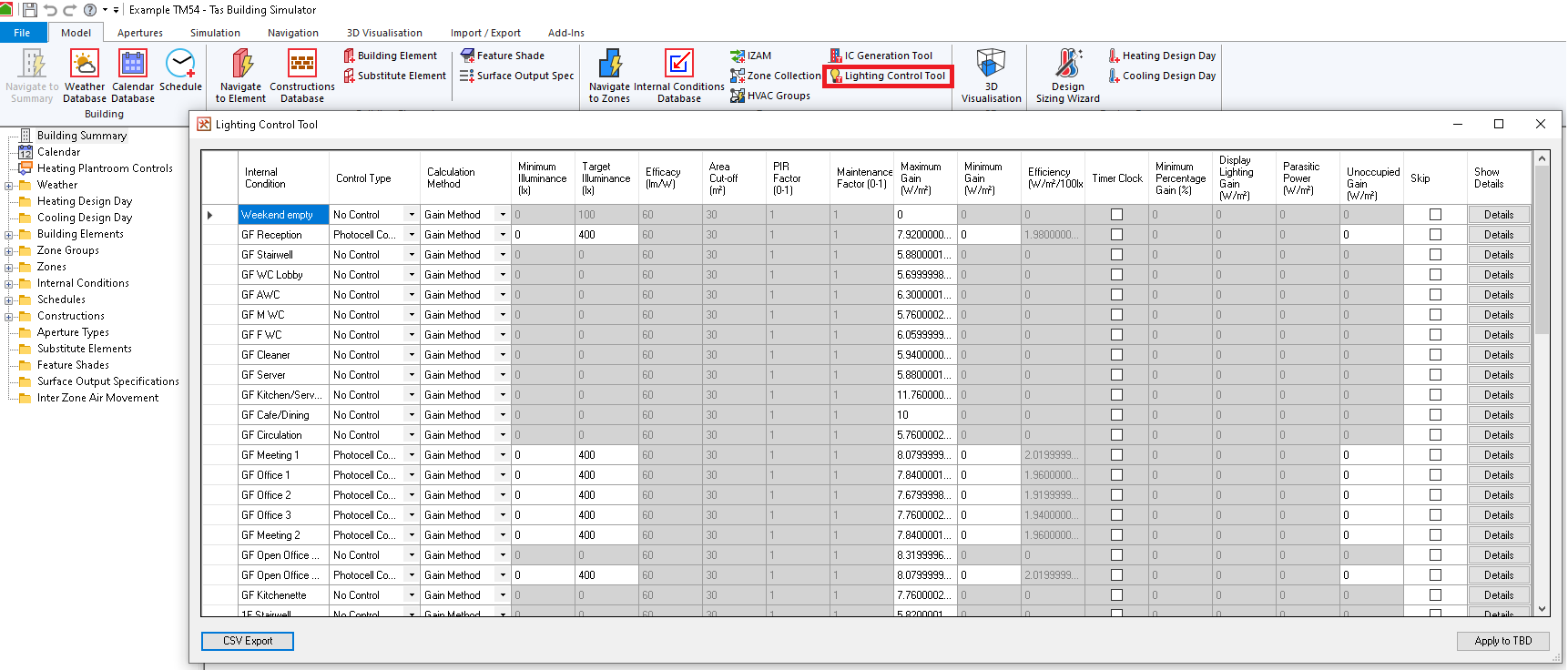
This tool allows lighting functions to be set up for multiple spaces much quicker, the data can be exported to EXCEL and worked on there if required. We have used this tool to set up the photocell controls in all of our perimeter office/meeting spaces and the reception. The lighting gains we’ve used in the TBD already allow for the factor from table 22 of the SBEM technical manual shown above.
Occupancy Gains – occupancy gains modelled should reflect the expected typical occupancy of the building, where necessary this should include for varying occupancy levels throughout the day. Our meeting rooms are unlikely to be occupied at all times and so a schedule has been applied to reflect the typical occupancy the rooms are expected to have on an occupied day.
Equipment gains – Equipment gains should reflect the expected typical levels, the gains used may well impact on cooling and heating demand and so should be modelled as accurately as possible. The equipment gains used will be reported as the small power usage for the space, gains should include for equipment that is run outside of occupied hours, our kitchen and kitchenettes for example have been run with a setback equipment gain when the building is not occupied to account for equipment that is run 24 hours such as fridges and freezers.
If you’re setting up a server room it’s important to account for if the server is likely to be on 24 hours and over the holidays even if the building is unoccupied. This should also be accounted for in the cooling schedule if the server room is cooled.
Equipment gains are often overestimated as the nameplate power rating of equipment is often much higher than the amount of power it will use on average. Although it’s often difficult to ascertain average power usage of equipment this should be taken into account where possible. If you were to model all of the kitchen equipment as on at maximum power for the whole day it’s likely that the small power usage will be dramatically overestimated.
If you have electrical usage you would like to include but don’t want to include for this as heat gain in the space this can be set up at a later stage in the Tas Systems file, this is useful for things like lifts where the motor is often located on the roof so the gain from the equipment shouldn’t be modelled as included in the thermal analysis. We’re going to be including for the energy usage due to the lift like this in our building.
Pollutant Generation – If you’re building has HVAC systems that are controlled on CO2 levels then the pollutant generation will have to be set up in the internal conditions to account for the build-up of CO2 in the space. Our building doesn’t have any ventilation systems that are controlled on CO2 levels so we’re not going to worry about setting up the pollutant generation per space.
DHW – The DHW demand should be accounted for in the internal conditions under the system parameters section, where DHW demand per space is specified in L/m2/day. All DHW demand in the building should be set up in the internal conditions, any demand not included in the internal conditions will not be accounted for.
If all DHW demand is met by the same system and the DHW demand is known for the building rather than on a zone by zone basis then all of this can be accounted for in one spaces internal condition, for example our building is expected to use 759,000L of DHW per year, the building is occupied for 253 days per year which equates to 3000L of DHW per day. The DHW is input in L/d/m2 so to include for all of the DHW in one space we need to divide the daily DHW usage by the space area and assign this value to that zones internal condition. We have assigned the DHW demand to the space GF Office Core, this space has an area of 180.78 so the DHW rate works out to be 16.59 L/d/m2. If you use this method it’s important to make sure that the internal condition used isn’t applied to any other zones as this will lead to increased DHW demand – This method should not be used if different areas of the building have the DHW demand met by different systems.
Heating and Cooling – The heating setpoints should be set up per space, as well as the radiant proportions of the heating and cooling emitters. It’s important to include for any pre-heat/cool if the building includes this. Our building is heated and cooled from an hour before occupancy, this is accounted for by the schedule applied to the heating and cooling setpoints. WCs and circulation spaces are heated by single panel radiators and so have been modelled with a radiant proportion of 0.5, all other spaces are heated by air side systems and so a radiant proportion of 0 has been used.
If heating and cooling capacities per space are known these can be input by selecting the zone, changing the sizing to no sizing and typing in the maximum capacity for the zone. If these aren’t known they can be left as sizing, this means that any heating/cooling demand required to keep the space to its setpoints will be met. To achieve the most accurate results we recommend that a full sizing design is carried out and the correct room loads are allowed for in the assessment.
Constructions – As with all Tas models the constructions should be set up as accurately as possible, modelling the material build-up of the constructions with the correct thermal mass will provide more accurate results.
Apertures – If your building utilises natural ventilation then the apertures should be set up accordingly, you should be careful when assigning the controls so that you’re not heating/cooling with the windows open as this could have a significant impact on the predicted heating and cooling usages. Our building is mechanically ventilated so we’re not setting up any apertures.
Setting up the Systems file
Systems is where we will set up the HVAC systems and simulate the buildings energy usage. To ensure the results are as accurate as they can be, the systems set up should reflect how the building will run in reality as closely as possible. If you feel you would like more help or guidance using systems than the worked example gives we would recommend you refer to the help documentation. We do also offer a Tas Systems training course, if you would like more information on this is can be found here.
We’re going to use the project wizard to set up some template systems and amend these where necessary. If you have carried out an L2 assessment on your building using Tas you can use the project wizard to import the tpdx file from the runs folder, doing so will bring across the HVAC systems and zone assignment from the L2 assessment. This is a great way to save having to set up all set up the systems and re-assign the zones again but it should be noted that the systems used in an L2 assessment are selected from a list of pre-set systems and so may need amending to represent how the actual systems in your building run.
To run the project wizard, open a new Tas systems file, this can be done from the applications in Tas manager, the new file will then have a project wizard button in the centre screen as shown below.
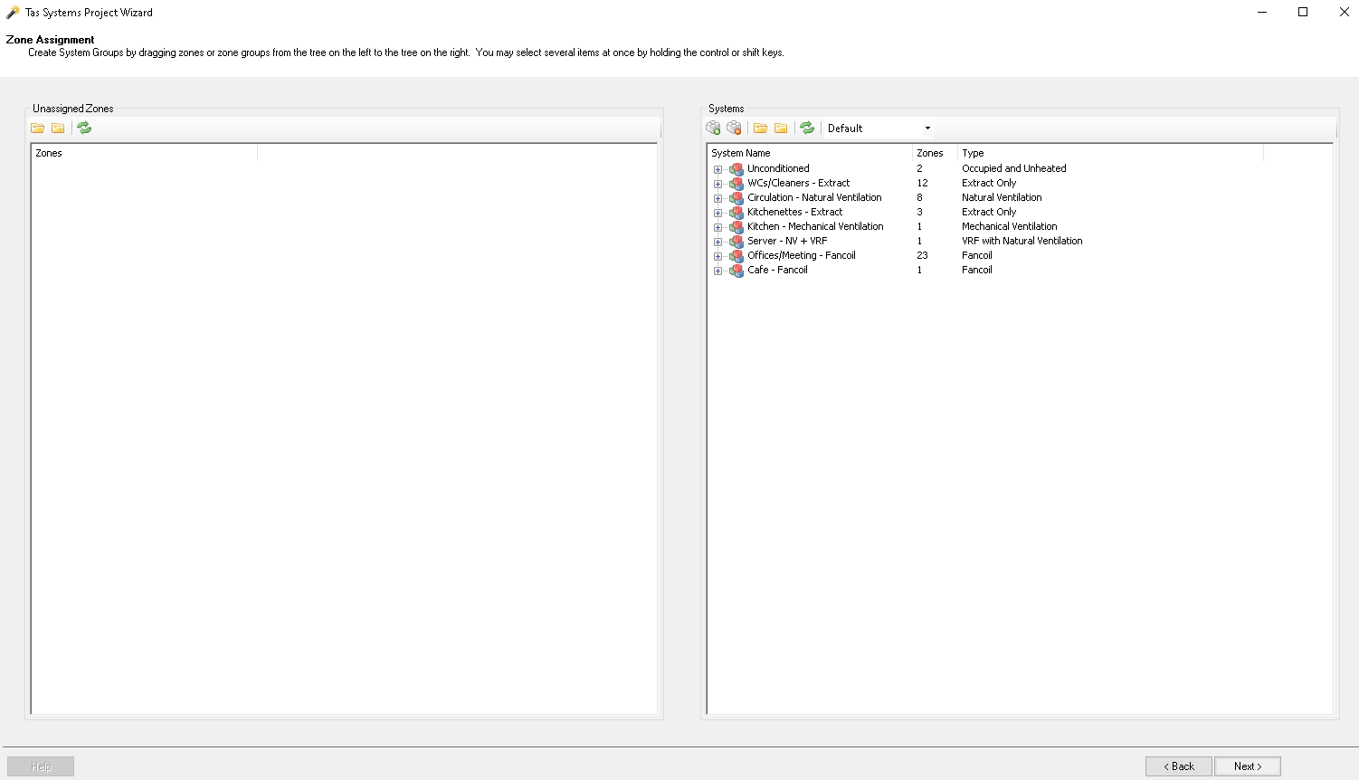
We’re going to create a new project and import the TSD data from the simulated TBD we just set up. We’ll then assign the zones to groups based on the HVAC system that serves them as shown below.
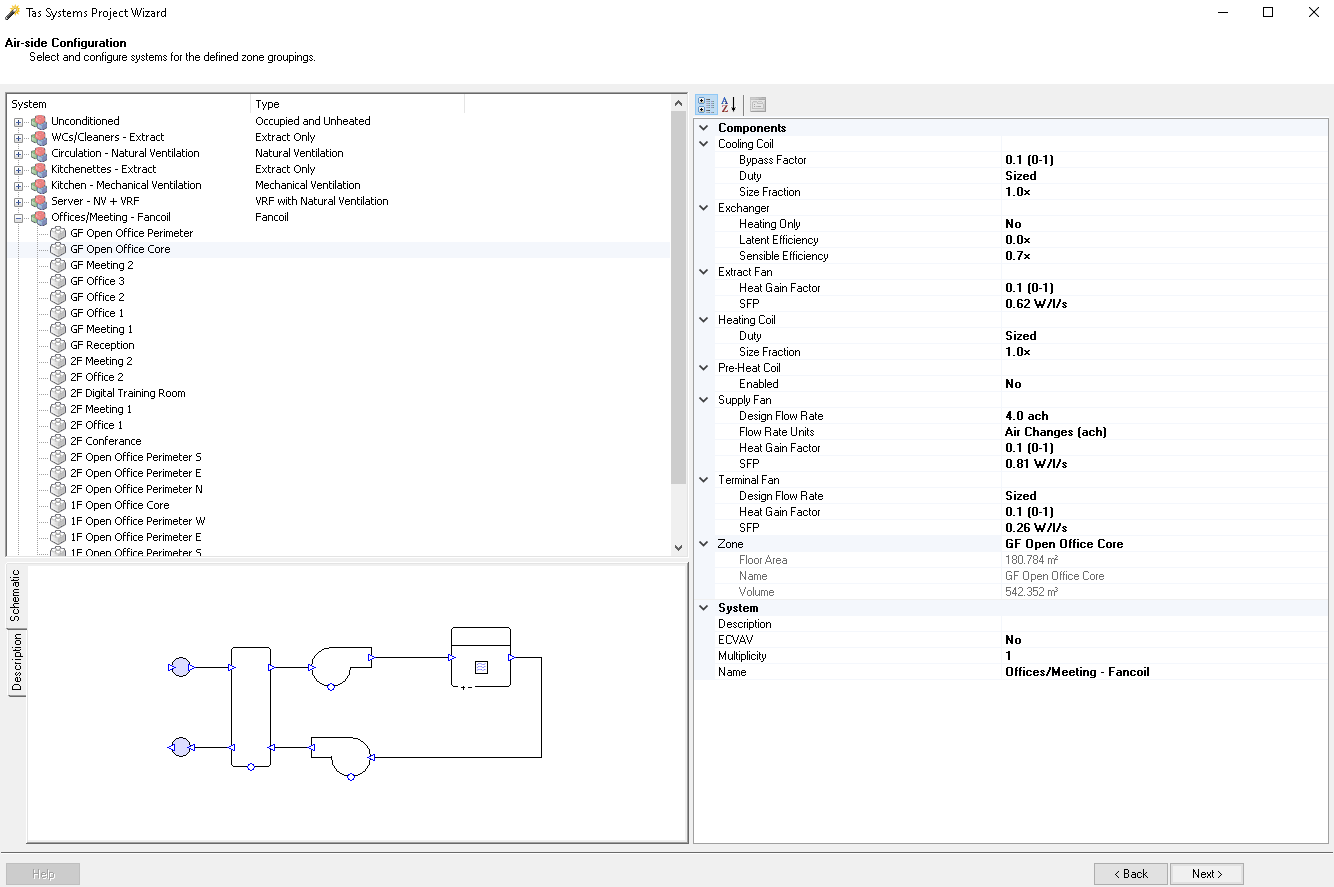
On the next page the HVAC systems are set up for each group by right clicking the group to assign one of the pre-set systems. A schematic of the selected system can be seen in the bottom left corner, this can be changed to a description of how the system operates by clicking on the description tab. The system details can then be set up by changing the fields on the right, these can be changed at a later stage if required. Component details can be set per space by expanding the tree view and selecting the required space, as shown below. If you’re setting up the heating and cooling capacities per space these can be input at this stage. If the template system will need amending then you may lose the flow data added per space here so it might be best to input this at a later stage.
On the next 2 pages heating and cooling circuits can be set up like in the Tas Studio when carrying out an L2 assessment. We’re setting up a Gas LTHW circuit for our fancoils, WCs, circulation spaces and kitchen/kitchenette. This circuit also serves a DHW tank which provides all the DHW demand for the building. We’re also setting up a VRF circuit for our server room. The efficiencies and duties of the boilers and chillers can also be set up here, these can also be changed at a later stage should the design change.
The next page of the project wizard is where the DHW circuits are set up, we’ve already set up a LTHW circuit with a DHW tank so we’re just going to assign all of the spaces to this circuit and set up the tank details and distribution efficiency. It’s important to note that the DHW demand is set up in the internal conditions, if you have more than one means of providing DHW then the DHW set in the internal conditions should be assigned such that the demand is split between the DHW heaters accordingly. For example if you have set up the DHW demand for the WCs in the office internal conditions (as is the case for the NCM internal conditions in part L) then you will need to ensure that the offices are assigned to the DHW circuit that provides the WCs DHW.
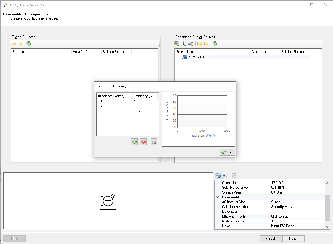
Renewables for the building can be set up on the next page of the project wizard. Our building has an 87m2 PV array on the roof so we’ve set this up here, the panel efficiency is 19.7% and this can be set up by clicking on the “Click to edit” button. If the AC inverter size is known this can also be input here. We’ve set up the PV array using the “Specify Values” calculation method, because we know our panels are completely unshaded, however if the building has shading that would affect the PV array then this should be accounted for by modelling the PV in the T3D 3D model along with the shade surface and using the calculation method “Use Zone Surface”.
On the next page fuel sources can be assigned to the components.
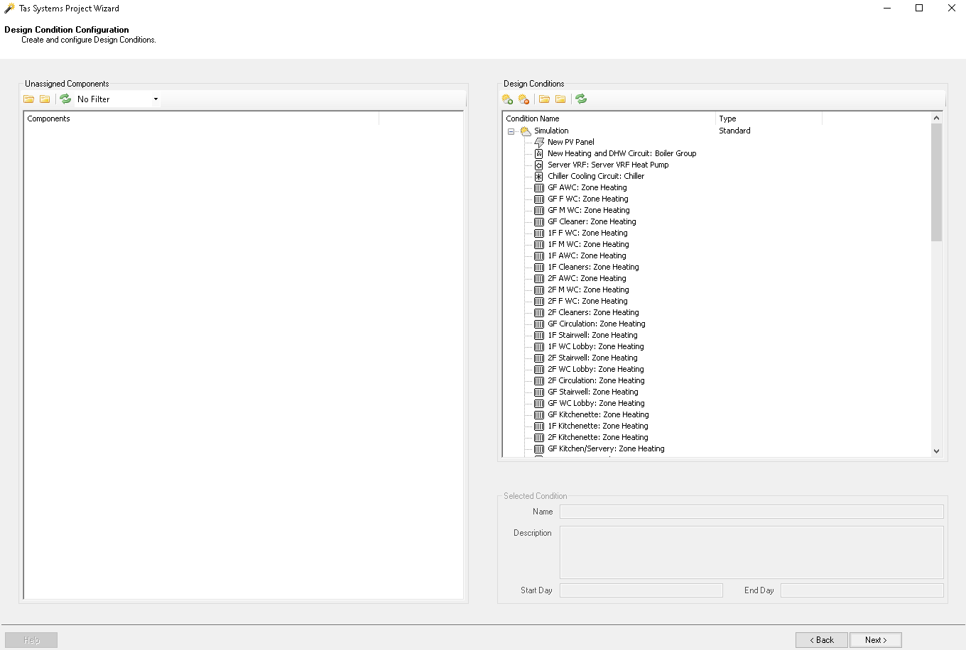
Finally design conditions can be set up for the systems, if you have design conditions set up in your TBD then these would appear in the list. For our building we’re just going to size everything on the yearlong simulation.
Next you can hit generate to finish the initial set up. As the systems are general template systems some of them may need editing to reflect your building, for example our Kitchen has been set up as mechanically ventilated, the default system includes heat recovery but our kitchen doesn’t have this. To remove the heat recovery from the system we’re going to select it from the tree view on the left, right click the system and select “ungroup”, the heat recovery unit can then be right clicked and deleted as shown below. Unfortunately un-grouping a system means that any previously entered flow data will have to be re-input.
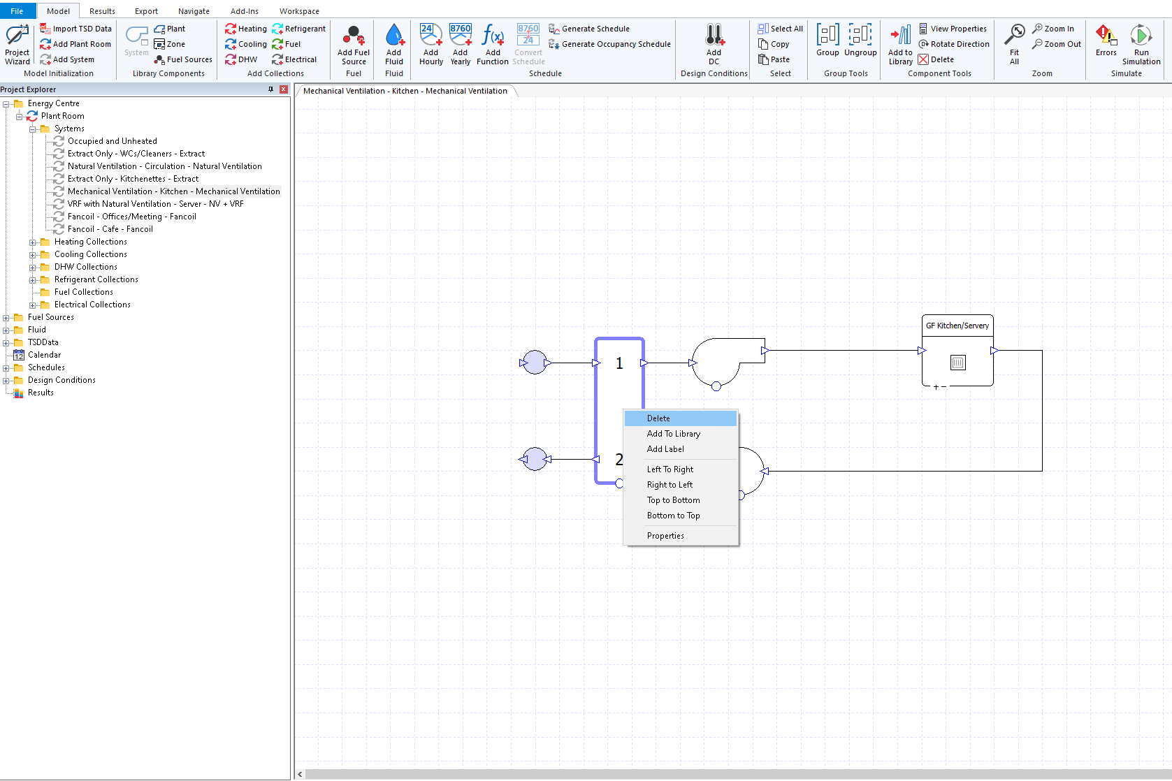
Once the heat recovery unit has been deleted the junctions will have to be re-connected to the fans, the whole system can then be selected and re-grouped. It’s important that the template systems are amended to reflect the actual building as accurately as possible, as modelling the systems incorrectly could have a significant impact on the results.
Checking schedules on systems and fans
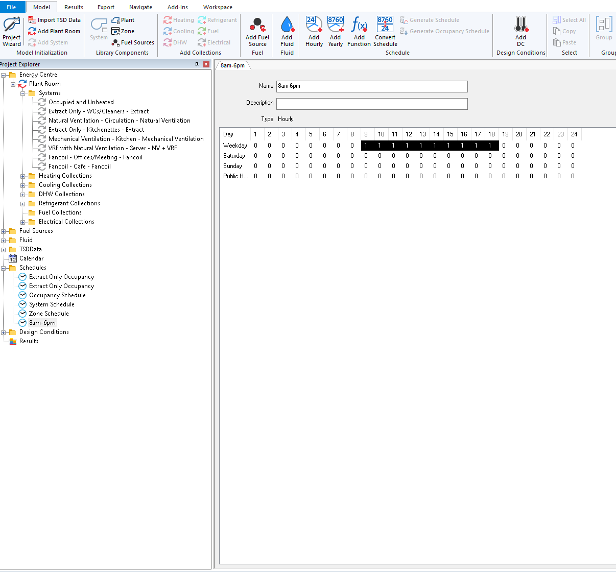
It’s worth checking the schedules applied to your system components as the software often defaults to occupancy for the schedule. For example our WCs fans have defaulted to be on when occupancy is present in the internal condition, as we didn’t set occupancy in the WCs we’ll have to update this schedule. To create a new one we right click on schedules in the tree view on the left and add an hourly schedule, our WC fans run from 8am-6pm on weekdays so we set this up as shown in the screenshot below
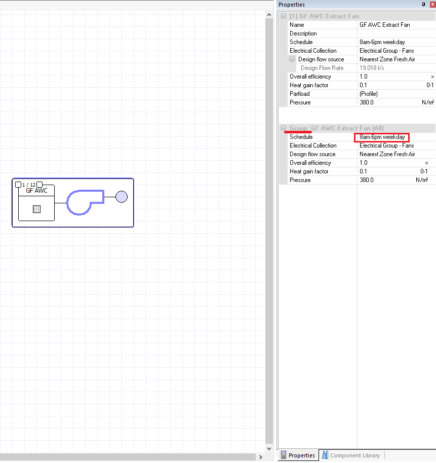
To assign this to our WC extract fans we select the system from the tree view and click on the fan in the grouped system, the properties for this can then be edited in the box on the right hand side of the screen. Properties can be changed for individual zones in a group, or for all zones in the group. Ensure you are applying the change to the entire group and not just the first zone in the group by changing the schedule highlighted below
Modelling additional energy usage as a load component
Now let’s add the lift energy usage to the model by using a load component, to do this we first create a new electrical collection and call it “Electrical Group – Lift”, to finish setting this up we right click on the new collection, assign the electrical source to grid supplied electricity and set its type to equipment. We then add a new system to the tplp file by right clicking the systems file and name this “Lift”. A Load component can then be dragged from the component list on the right hand side of the screen and dropped into the system, the properties for this can be edited by right clicking the component and selecting properties. We’re going to assign it to the lift collection.
As the software works in hourly time blocks we need to look at the average wattage use of the lift for an hour, for example if a lift uses 1000W when running but only runs for 15minutes of the hour than the average wattage use of the lift over the hour would be 250W, let’s call this the “hourly wattage”. The term “peak hourly wattage” used below means the peak of the hourly wattages for the lift.
To assign the load to the component we select the “Load” tab in the properties. We want to set up our lift such that it uses its peak hourly wattage from 8am-9pm and 5pm-6pm, 60% of this for 2 hours over lunch and 10% for the remainder of the day. To do this we calculate the hourly wattage values and input them in the schedule as shown below. The ‘Value’ shown will not be used as the hourly profile values override this.
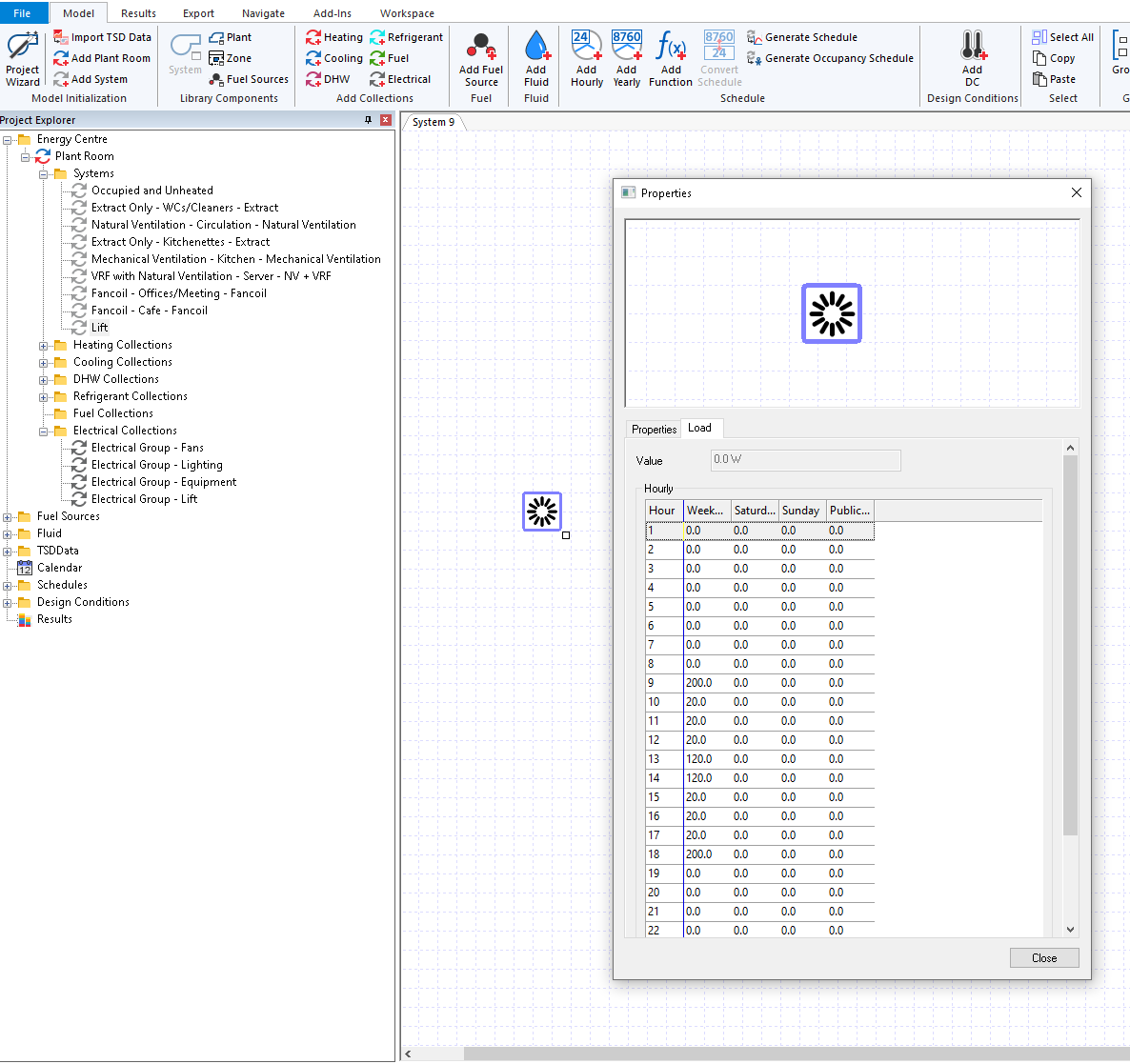
If you want to know more about calculating the peak hourly wattage for the lift TM54 offers some guidance on calculating the energy usage of lifts. If you need to account for external lighting or any other additional energy usages in your building this can also be done using a load component.
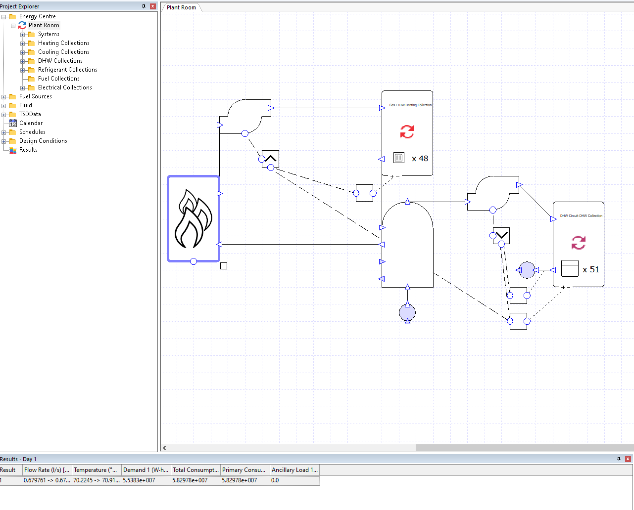
Setting up the plant room
If you have plant details such as LTHW & DHW setpoints, boiler & heat pump capacities design pressure drops etc. these can be input for the relative components by selecting the plant room from the tree view and amending the properties of the components. The greater detail the plant can be modelled to the more accurate the results should be for the assessment.
Once we’re happy with how everything has been set up we can simulate our systems file by right clicking on the energy centre folder in the tree view and clicking simulate.
Checking the systems file
It’s always good practice to check your systems are behaving as expected once the model has been simulated. A great place to start is by checking for any errors or warnings in your plant room and in each of your systems. To do this simply click on plant room or one of your systems in the tree view and look at the box in the bottom right hand side of your screen, you can check for both errors and simulation events by clicking on the relevant tabs in this box. If any of your systems or plant have errors or warnings then these should be checked.
Some warnings can be ignored, for example if you have set up the heating and cooling capacities per space and there are some spaces with a couple of unmet hours this may not be a concern, it could be that the heating doesn’t quite reach the setpoint for the first hour after being unoccupied over the weekend for example. If your building has a significant number of unmet hours however this should be looked into as the simulation won’t be accounting for maintaining the specified heating/cooling setpoints. It could be that the heating/cooling capacities have been input incorrectly or the systems have been undersized, either in terms of the room loads or the fresh air loads. Reasons for this may be that the design condition used for sizing was not as onerous as the dynamic simulation, for example.
Another good way to check your plant and systems components are behaving as expected is to simply highlight these and look at the results for a few days, this way you can quickly check if fans are running when they should be and that spaces are being maintained to the heating/cooling setpoints at the correct times. Let’s double check the WC fans are running when expected as we assigned a schedule to these, we right click the fan in the systems and then can look at the results in the bottom left box:
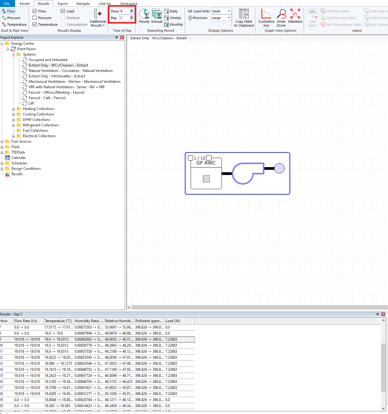
For day 2 we can see that our fan is running from 8am-6pm as expected, the day and time of the results shown can be changed in the ribbon as highlighted in the screenshot above. If you find any of your systems aren’t running when you expect them to you will have to check they’re set up correctly.
Outputting and reporting results
Once you’ve checked over your systems and are happy that they are running as expected you can start outputting results from the software. Selecting results from the tree view brings up the annual demand and consumption for the building as shown in the screenshot below.
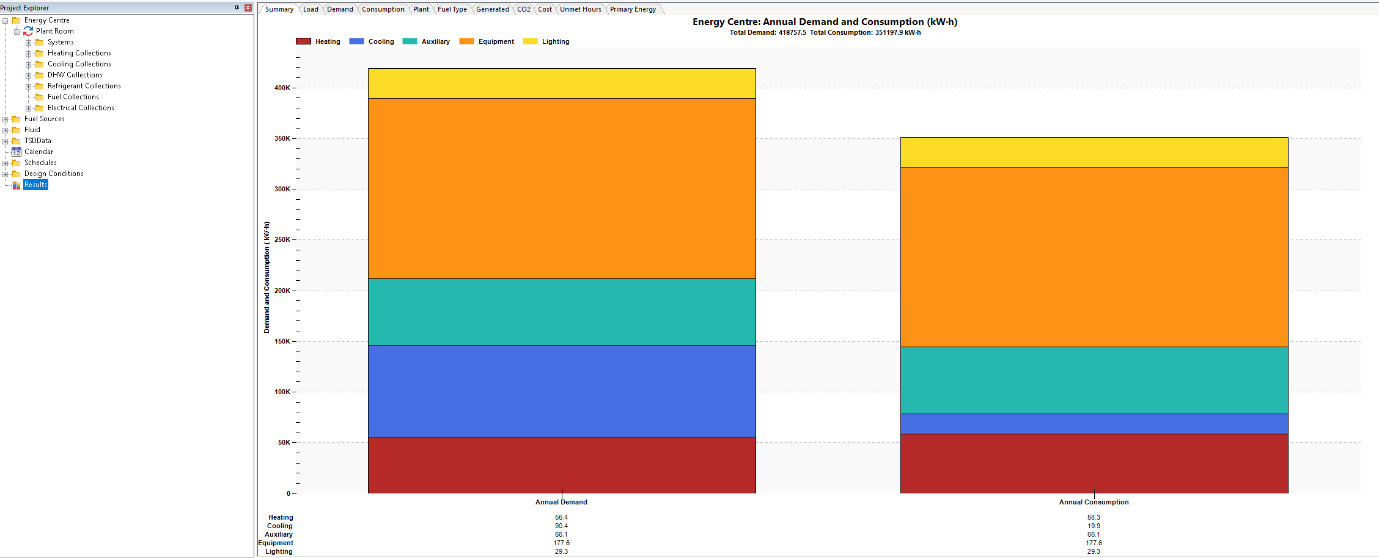
DHW is included within the heating category, the results data can be copied to your clipboard and pasted to EXCEL or elsewhere. If results are needed on a monthly basis selecting the demand and consumption tabs at the top of the results graph provides the respective results on a month by month basis. Selecting the plant tab provides a further breakdown of consumption results, including separate consumptions for each electrical group set up:
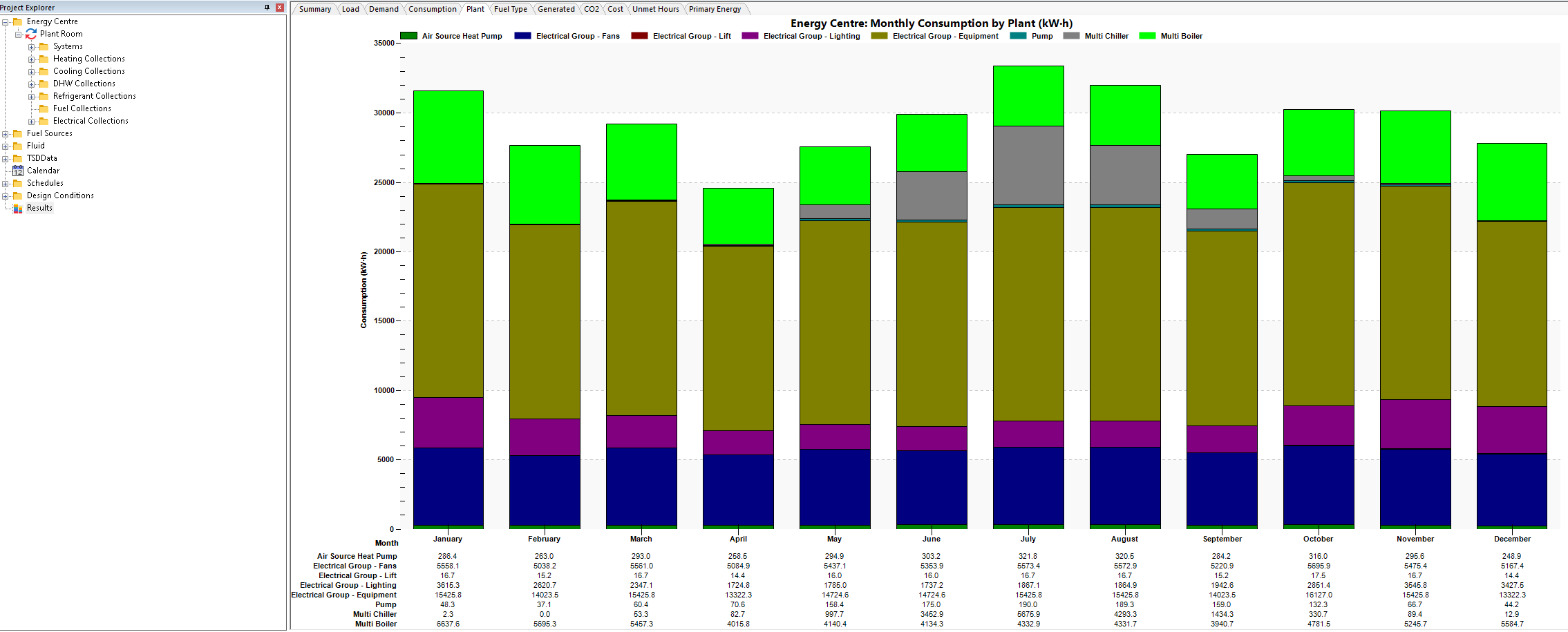
The annual plant breakdown can be displayed by right clicking the results and selecting Annual, all results can also be displayed in kWh/ m2 by right clicking and selecting divide by floor area. The generated tab shows the energy produced by any renewables modelled.
We want to report DHW consumption and Heating consumption separately but this isnt a native output from Tas Systems because a boiler can meet both heating & DHW at the same time, so the load on the boiler is combined. However we can calculate it. To do this we’re going to calculate the DHW consumption we’re going to look at the annual results for the LTHW with DHW tank circuit. To do this we select this system in the plant room, right click the results in the bottom left of the screen and change the period to annual.
We first have to calculate the DHW demand, we can do this using the equation DHW demand = boiler demand – (LTHW heating collection demand/LTHW heating collection distribution efficiency). To get the annual demand for the LTHW heating collection we simply click on this and look at the annual demand on this collection, this must be divided by the distribution efficiency to account for distribution losses on the circuit. Once we have calculated the DHW demand we can then divide this by the boiler efficiency to calculate the DHW consumption. The method for separating the DHW demand from the heating demand may vary depending on the system providing the DHW, if you’re unsure how to separate the heating and DHW demand for your system then you should contact support for more guidance on this.
The annual results for our building are as follows:
Heating | DHW | Cooling | Auxiliary | Equipment | Lighting | |
Annual Demand (kWh) | 8025.5 | 47357.5 | 90385.7 | 66070.3 | 177589.2 | 29329.4 |
Annual Consumption (kWh) | 8461.3 | 49850.0 | 19897.8 | 66070.3 | 177589.2 | 29329.4 |
Here equipment includes the lift usage, if this is required separately this is easily obtainable by looking at the plant breakdown results.
Runs for error margins – changing weather data and scenario runs
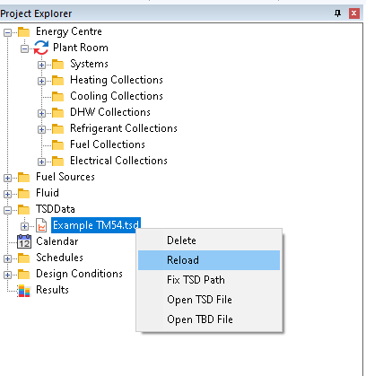
TM54 states that the buildings performance with future weather data should be analysed, this is useful for understanding how the building will perform with more extreme weather data and in the future. Once the model has been set up, looking at results for different weather data is easy but it’s probably best to make a copy of your files and keep them separate so that it’s clear which weather files have been used in each set of files. To get results for a different weather file, change the weather data in the TBD and re-simulate this to provide a new TSD. Then re-load the TSD corresponding to the new weather data from the systems file by expanding the TSD data folder in the tree view and right clicking on the TSD as shown below.
The TM54 report should also include error margins on the results reported, the error margins shouldn’t simply be based on consumption plus/minus 10% but should reflect different running scenarios for your building. For example when looking at the possible variation in heating consumption you shouldn’t simply increase and decrease the calculated value by 10% but should consider some possible scenarios that would increase the heating consumption, maybe occupants are likely to increase the setpoint if they have the opportunity to do so, maybe the heating will be used for a longer period due to occupants arriving early/staying late, maybe equipment gains have been overestimated and so in reality heating demand will be slightly higher. Models should be set up to test the impact of these different scenarios on the results.
The scenario modelling should account for variations with how the building is run by allowing for error margins to be included in the results. When setting up the different scenarios it’s important to consider how the changes will impact different energy usage categories individually and care should be taken so that the scenarios don’t cancel each other out. For example increasing the modelled equipment gains could increase the cooling energy consumption so this change shouldn’t be investigated alongside testing the effect of increasing the cooling setpoint. It may well be necessary to set up a number of different scenario models to look at the effects of changes to each energy usage category separately.
TM54 is a complex assessment and carrying one out on a complex building can seem a daunting task but by utilising the tools available through Tas Building Designer you can carry out a fast, robust and reliable calculation in no time. With the increasing threat of climate change it’s more important than ever that we work towards making our buildings as efficient as possible and reduce energy consumption where we can. If you need a TM54 assessment carrying out on a building but feel you need some assistance with some of or all of the process, our constancy team are more than happy to help and can be contacted by email consultancy@edsl.net.